|
A New View of Statistics | |
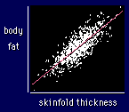
 Let's return to our example of skinfolds
and body fat. The correlation coefficient (r) indicates the extent to which the
pairs of numbers for these two variables lie on a straight line. The correlation
for this example is 0.9. If the trend went downward rather than upwards, the correlation
would be -0.9. For perfect linearity, r = ±1. If there is no linear trend
at all--for example, if there is a random scatter of points--the value of r is
close to zero. Points distributed evenly around a circle would also give a correlation
of near zero, because there would be no overall linear trend.
Which brings us to the question of how big a correlation has to be before it means anything. Correlations of less than 0.1 are as good as garbage. The correlation shown, 0.9, is very strong. Correlations have to be this good before you can talk about accurately predicting the Y value from the X value, especially when you want to use the result of the prediction to rank people. You can understand that by looking at the scatter of body fat about the line for a given value of skinfold thickness (the standard error of the estimate): it's still quite large, even for this correlation of 0.9. More on magnitudes of correlations shortly.
The details of calculation of correlations needn't concern us, because the stats packages do all that for us. But you should learn that the correlation between two variables X and Y is defined as the covariance of X with Y (covarXY) divided by the product of the standard deviation of X (stdevX) and the standard deviation of Y (stdevY):
r = covarXY/(stdevX·stdevY).
We've already met the variance: it's the mean value of all the differences from the mean multiplied by themselves (=squared). The covariance is similar: it's the mean value of all the pairs of differences from the mean for X multiplied by the differences from the mean for Y. If X and Y aren't closely related to each other, they don't co-vary, so the covariance is small, so the correlation is small. If X and Y are closely related, covarXY turns out to be almost the same as stdevX·stdevY, so the correlation is almost 1.
There are several important kinds of correlation, differing in the details of calculation. The most common is known as the Pearson (after a famous statistician). An older name is the product-moment correlation, which refers to the way it's calculated. The Pearson is what you get when you fit the best straight line to a set of points, such that the points are closest to the line when measured in the Y direction--the usual least-squares line, in other words. The topic of fitting lines and curves comes up in more detail later.
By the way, if the X and Y variables have the same standard deviation, the slope of the line is the correlation coefficient. Or to put it another way, if you normalize the X and Y variables by dividing them by their standard deviations, the slope of the line is the correlation coefficient.
Two more important kinds of correlation are the Spearman
and intraclass correlation coefficient (ICC). The Spearman
comes up later in connection with
non-parametric tests. The ICC is used as
a measure of the reliability of a
variable, whereas the Pearson is used for the
validity of the variable. The values of the
Pearson, Spearman, and intraclass correlation coefficients are
usually similar for the same set of data.
The strength of the relationship between X and Y is sometimes
expressed by squaring the correlation coefficient and multiplying by
100. The resulting statistic is known as variance explained
(or R2). Example: a
correlation of 0.5 means 0.52x100 =
25% of the variance in Y is "explained" or predicted by the X
variable. The reason why squaring a correlation results in a
proportion of variance is a consequence of the way correlation is
defined. You don't need to know the details right now.
See later.
Next up is another effect statistic,
relative frequency.
Go to: Next · Previous · Contents · Search
· Home
webmaster=AT=newstats.org
Last updated 10 Dec 00