A New View of Statistics	© 1998 Will G Hopkins
Go to: Previous · Contents · Search · Home

REPEATED MEASURES WITH PROC MIXED:
INDIVIDUAL DIFFERENCES, AND COVARIATES

/*
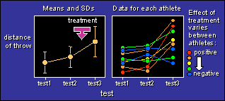
Repeated measures, with one between-subjects effect (grp) with
two levels (exptal and control) and one one within-subject effect
(test) with three levels.  The exptal group has a variable response
to the treatment, in the third test.
 
The individual differences are taken out for the first analysis.
The second analysis includes the individual differences.
The third analysis includes a covariate that accounts for the
individual differences.
 
See the output.
*/
 
options linesize=70;
options pagesize=32;
 
/*
Generates data for 12 athletes with true mean=60, between SD=5 
(excluding within SD), within SD=1.
An experimental effect of 3.0 is added in the third test. It varies
randomly between subjects with an SD of 2.0, to represent individual
differences. This variability is introduced via the variable indiff,
which is the covariate in the third analysis.
Try 200 athletes if you want to see these effects clearly.
 
You can ignore the mean of 60 and think of the experimental effect and
the variabilities as percents.
*/
 
data dat1;
n_per_gp=12; *sample size per group;
seed=12345; *seed to generate this output;
*seed=0; *use this seed to generate different samples every time;
grp="control";
do athlete=1 to n_per_gp;
  true=60+5*rannor(seed);
  indiff=rannor(seed); *needed for analysis with covariate;
  dist1=true+1*rannor(seed);
  dist2=true+1*rannor(seed);
  dist3=true+1*rannor(seed); *indiff NOT added in;
  output;
end;
grp="exptal";
do athlete=n_per_gp+1 to 2*n_per_gp;
  true=5*rannor(seed);
  indiff=rannor(seed); *for analysis with covariate;
  dist1=true+1*rannor(seed);
  dist2=true+1*rannor(seed);
  dist3=true+3+2*indiff+1*rannor(seed); *indiff added in;
  output;
end;
run;
 
*Converts data for proc mixed;
data dat2;
set dat1;
v33=0; *for Satterthwaite confidence limits;
distance=dist1; test=1; output;
distance=dist2; test=2; output;
if grp="exptal" then v33 = 1; else v33 = 0;
distance=dist3; test=3; output;
 
*Data with no individ diffs;
data dat3;
set dat2;
if grp="exptal" and test=3 then distance=distance-2*indiff;
 
*Generates matrix of covariance parameters;
*for Wald confidence limits;
data matrix;
input parm row col1-col3;
datalines;
1 1  1 1 1
1 2  1 1 1
1 3  1 1 1
2 1  1 0 0
2 2  0 1 0
2 3  0 0 1
3 3  0 0 1
 
 
/*
FIRST analysis
Wald estimates of CLs of variances.
Use when individual diffs < within error.
Currently this analysis estimates but does not compare
individual differences in the exptal and control groups.
*/
proc mixed data=dat3 covtest cl;
class athlete grp test;
model distance=grp test grp*test;
repeated / subject=athlete type=lin(3) 
         ldata=matrix group=grp;
parms (25) (1) (0) (25) (1) (0);
estimate 'grp*test 2-1' grp*test 1 -1 0  -1 1 0/cl;
estimate 'grp*test 3-2' grp*test 0 1 -1  0 -1 1/cl;
title "WITHOUT individual differences";
 
/*
SECOND analysis
Satterthwaite estimates of CLs of variances.
Use when individual diffs >= within error.
Currently this analysis assumes no individual differences
in the control group.
*/
proc mixed data=dat2 covtest cl;
class athlete grp test;
model distance=grp test grp*test;
random int v33 / subject=athlete;
estimate 'grp*test 2-1' grp*test 1 -1 0 -1 1 0/cl;
estimate 'grp*test 3-2' grp*test 0 1 -1 0 -1 1/cl;
title "WITH individual differences";
 
/*
THIRD analysis
Using a covariate to account for indiv. diffs.
This analysis does a full comparison of the value
of the covariate in exptal and control groups.
*/
proc mixed data=dat2 covtest cl;
class athlete grp test;
model distance=indiff|grp|test; *full model;
repeated / subject=athlete type=lin(3) 
         ldata=matrix group=grp;
parms (25) (1) (0) (25) (1) (0);
estimate 'grp*test 2-1' grp*test 1 -1 0  -1 1 0/cl;
estimate 'grp*test 3-2' grp*test 0 1 -1  0 -1 1/cl;
estimate 'indiff*grp*test 2-1' indiff*grp*test 1 -1 0 -1 1 0/cl;
estimate 'indiff*grp*test 3-2' indiff*grp*test 0 1 -1 0 -1 1/cl;
title "Including a covariate";
run;